Farey Graphs

Over the summer of 2018, I was a part of the ICERM REU where I worked on a project about Farey Graphs (joint work with J. Gaster, E. Rexer, Z. Riell, and Y. Xiao). We made a lot of beautiful pictures and proved some interesting results that I want to show off and say a little about.

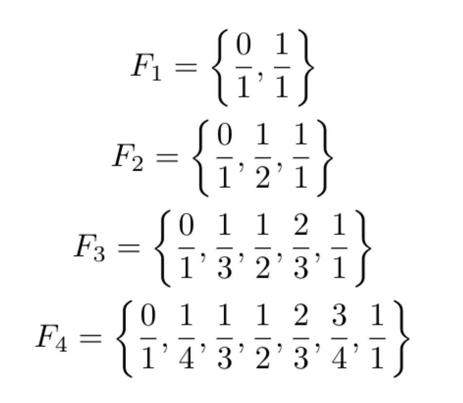
The $n$ th Farey sequence $F_n$ is a list of fractions named after Sir John Farey, a British mathematician who was not actually the first to discover them. The original discoverer, Charles Haros, wrote about them 14 years prior (an example of Stigler’s Law) unbeknownst to Farey. The first few sequences are as follows:

To define the terms of each sequence, we let the operation $\oplus$ between two rational numbers be

$\displaystyle \frac{a}{b} \oplus \frac{c}{d} = \frac{a+b}{c+d}.$

One produces $F_{n+1}$ from $F_n$ by inserting between each two consecutive entries $a/b$ and $c/d$ of $F_n$ the rational $a/b \oplus c/d$ . It turns out that if we continue this process infinitely, we will reach every rational between 0 and 1 having no repeated entries.

To understand this sequence geometrically, we consider a graph $G = (V,E)$ with vertex set $V = \mathbb{Q} \cap [0,1]$ . A pair of rational numbers $(v,w)$ forms an edge in $E$ if, in some $F_n$ , $v$ and $w$ appear as consecutive entries.

A subgraph of G depicting the terms of 9th Farey sequence. Image via Wikimedia Commons distributed under CC BY-SA 4.0 license.

We can extend this graph to be defined on all of $\mathbb{Q}$ plus a ‘point at infinity’ which we denote by $1/0$ . Adding this point yields a highly symmetric graph that can be embedded into hyperbolic space. We define the edge set of our new extended graph $\mathcal{F} = (V,E)$ by defining $(p/q, s/t) \in E$ whenever we have

$\left| \text{det} \begin{bmatrix} p & s \\ q & t \end{bmatrix} \right| = 1$

One can check that we recover $G$ as a subgraph of $\mathcal{F}$ . Using Poincaire’s disc model of hyperbolic space, we can visualize this graph as seen below.

In the disc model, the real numbers are wrapped around the boundary of a disc and glued at the top by the point at infinity. Hence the vertices of our graph form a dense subset of the boundary and the edges connecting them are geodesic arcs through hyperbolic space. The graph $\mathcal{F}$ actually triangulates hyperbolic space, since the embedding has no two edges intersecting and each edge is a side of two hyperbolic triangles.

The definition of $\mathcal{F}$ naturally leads us to a generalization: instead of having the above determinant equal to $\pm 1$ we define the edge set of $\mathcal{F}_k$ to have edges when the determinant is $\pm k$ . We call the $k$ th graph in this family the $k$ -Farey graph and depict $\mathcal{F}_2$ below.

Our team explored the connectivity of these graphs and made the following discovery: the number of connected components of $\mathcal{F}_k$ is given by

$b_0(\mathcal{F}_k) = \begin{cases} p^{\ell -1}(p + 1) & k = p^{\ell} \\ \infty & \text{otherwise} \end{cases}$

where $p$ is a prime number and $\ell > 0$ is a positive integer. For example $\mathcal{F}_7$ has eight connected components shown below, where each is colored by its corresponding component.

Moreover, each connected component of $\mathcal{F}_7$ is a planar graph; one such component is shown below.

We also have results on the automorphism groups, chromatic numbers and dual graphs of the $\mathcal{F}_k$ , so check out the paper on arxiv to learn more!

Below is a gallery of some $\mathcal{F}_k$ ‘s, all of which were made in Mathematica by me. Notice anything patterns for certain integers? Let me know!